I built Gage to inspect why a part image received an anomaly decision. I put the score beside a normal reference and a difference map, then added a way to record a reviewer’s correction.
Local visual anomaly inspection against normal references
My role
I built the reference comparisons, experiment and local review interface.
Year
2026
Contents
Making a part inspection reviewable
I built Gage around a practical inspection question: if a system flags a part, what can I show someone who needs to check that decision? A score gives a decision boundary, but reviewing a mark or an edge also needs an image and a comparison. I wanted to keep that explanation close to the result.
I chose one generated shape, a rectangular plate with a circular opening, and a local Python application running on CPU. That scope let me build the complete path from normal examples to an inspection screen. I could follow a prediction back to its reference, measure its mistakes and save a correction without changing the experiment underneath it.
Starting with a normal part that raises an alarm
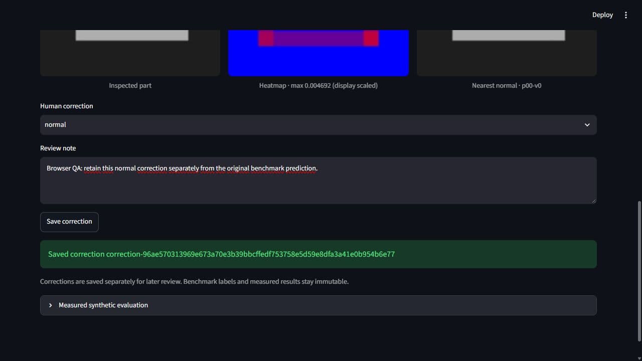
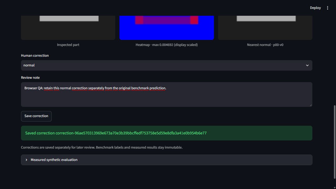
The default replay opens p20-v0, a normal image that the patch method flags as anomalous. Its score is about 0.004646 against a saved threshold of 0.003627. The returned normal comparison is p00-v0. I kept this example because it gives the reviewer something concrete to investigate immediately.
The screen shows the inspected part beside its heatmap and reference. I can look at the activated regions, choose a normal correction and attach a note. Saving that review leaves the original prediction available. It also gives me a useful question for development: is this alarm responding to a defect, or to a difference that my normal bank represents poorly?
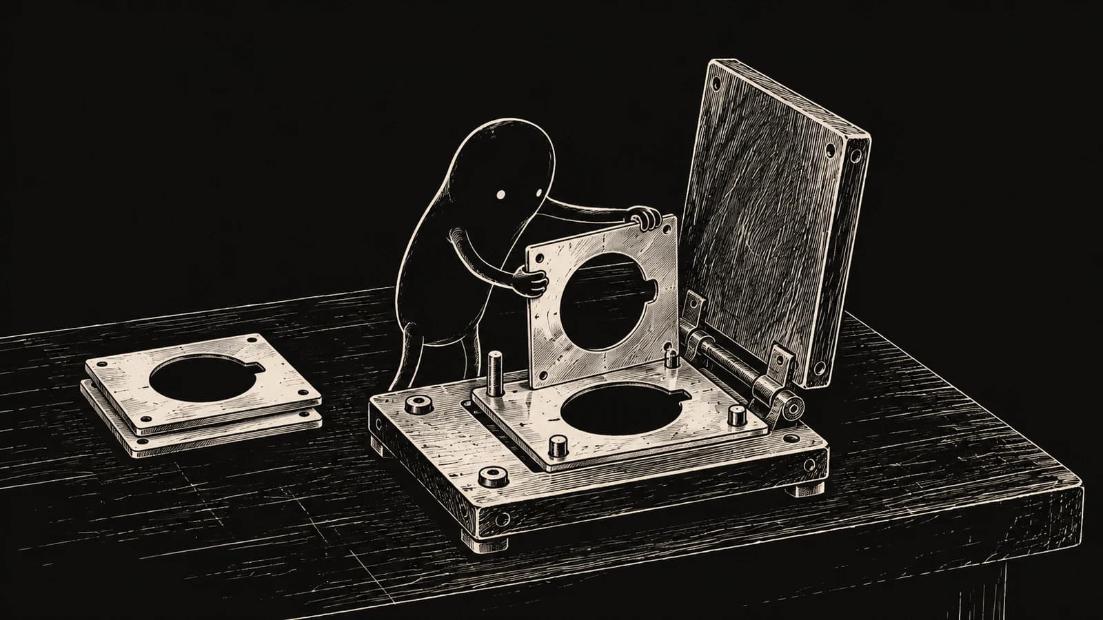
I illustrated reference comparison through a creature aligning a part with its stencil.
Following the inspection through one screen
I organized the Streamlit interface around two inputs: replay an existing fixture image or upload a generated PNG. The active backend, saved bank identity and validation threshold appear before inspection. Pressing Inspect image clears the previous result before starting another comparison, so a failed request cannot leave an earlier success looking current.
The result places score and decision above three image columns. I scale the heatmap colors for display while retaining the original values for scoring. Correction controls sit below that evidence, followed by the saved evaluation panel. An empty upload produces an actionable error. A missing reference preview produces a warning beside the valid score, allowing the review to continue.
Application screens
1 / 2
I inspected the alarm alongside its heatmap and reference, then saved the correction separately.
I generated 90 RGB images with defect masks across 30 part groups, using seed 42. Twelve groups supplied 36 normal training views. Eight supplied 24 validation images, and ten supplied 30 test images. Keeping a part group inside one split was intended to separate the views used for fitting and measurement.
Checking decoded image contents exposed a weakness in that separation. The files contained only 83 distinct images, including three normal test images that exactly matched training content. I preserved the original population and recorded those collisions. The nominal results belong to this small fixture; cleaning duplicates after seeing the outcome would require a separately identified experiment.
Keeping image evidence separate from evaluation labels
I separated loading, scoring, evaluation and review into modules that the CLI and interface can share. Fitting receives normal training pixels. Prediction receives an RGB image and saved reference bank, returning a score, heatmap and reference ID. Labels and defect masks stay in evaluation, where I can compare predictions with expected regions.
Saved numerical banks carry training IDs and configuration identities. Loading checks their shapes, finite values and checksums with pickle disabled. Replay first enumerates IDs; inspecting an item resolves only that image. This structure lets an upload use the saved bank even when replay metadata is unavailable. The interface adds evidence previews and review controls around that shared scoring operation.
Establishing a pixel comparison I could explain
My baseline converts each image to grayscale and finds the normal training image with the smallest average absolute difference. The resulting pixel differences form the heatmap. I average its largest one percent of values to obtain the image score, so a small changed region can influence the decision without being diluted across the entire plate.
I kept alignment and resizing unchanged. That makes the baseline easy to inspect: a displaced edge or brightness change remains visible in the map. It also makes its assumptions explicit. The comparison expects matching geometry and reasonably consistent illumination, which gave me specific conditions to test once the nominal inspection path worked.
Trading exact position for patch matching
For the second method, I divided each 96×96 image into 8×8 patches. Each patch has eight handcrafted features: RGB means and standard deviations, plus horizontal and vertical grayscale gradient magnitudes. These describe average appearance and local variation without fitting a neural network.
A query patch searches every normal training patch, including patches at other locations. I repeat its nearest distance across the corresponding map cell. The displayed reference uses an aggregate whole-image comparison, so individual cells can obtain their closest match from different normal images. That distinction matters when reading the screen: the single reference is a useful comparison, while the map summarizes a larger bank. Coarse cells also limit thin-boundary detail.
Choosing operating points before looking at test results
A continuous score needs a threshold before it becomes an alarm. I selected image thresholds on validation data by maximizing anomaly recall while keeping observed false positives at or below ten percent. With only eight normal validation images, one false alarm would already mean 12.5 percent. The rule therefore permitted zero observed false alarms.
I saved those choices before scoring the test images. Pixel thresholds were selected separately for region overlap. This lets me ask two different questions: did the image raise an alarm, and did its map cover the defect? I also saved the stress recipe with the choices, preserving the conditions behind each reported result.
Reading ranking, alarms and regions separately
The nominal test contains ten normal images and twenty anomalies. Patch AUROC was 1, meaning its scores ranked every anomaly above every normal in this population. At the frozen decision threshold it caught all twenty anomalies and also flagged three of the ten normals. Ranking quality and the chosen operating point gave different impressions of the same method.
The residual baseline had AUROC 0.9075 but caught zero of twenty anomalies at its threshold. Its defect-region overlap was much better: macro pixel IoU was about 0.893, compared with 0.266 for patches. IoU measures the intersection of predicted and expected regions relative to their union. Averaging it per anomalous image keeps that localization question separate from the alarm.
Changing lighting and position without changing thresholds
I multiplied brightness by 0.7 and 1.3, then shifted images four pixels in each horizontal direction. These variants come from the same thirty test parents. I retained their identities so the additional predictions remain recognizable as paired transformations.
The patch method flagged every normal image in both stress families. Under lighting changes, both methods' macro pixel IoU fell to about 0.0069. Broad differences overwhelmed the region comparison. The baseline also missed the nominal anomaly p20-v1 despite a useful residual map: its image score stayed below the frozen threshold. I retained these failures because they identify separate work on illumination, registration and decision selection that a stronger nominal score would have concealed.
Preserving the evidence behind a review
A reference filename alone cannot establish that the displayed pixels are the ones used during fitting. I verify original training dimensions and the ordered RGB content hash before showing the preview. If that check fails, I withhold the reference image and explain why. Scoring and correction remain available when their saved artifacts are valid.
Corrections go into a separate local JSONL log with image and bank identities. Repeating an identical save returns the same correction ID; changing the decision or note adds a record. I validate existing entries before appending. This gives the single-user review flow a clear history while keeping benchmark labels, metrics and saved predictions intact.
What I would change in the next experiment
The comparison changed the order of work I would do next. I would first generate a new, content-deduplicated dataset with more normal validation examples, defining part groups before producing views. Lighting and position variation need their own controls so I can distinguish damage from acquisition changes when selecting an operating point.
Then I would compare registration or intensity normalization on validation data. Smaller or overlapping patches could test boundary detail; frozen learned features would need a separate measured adapter. I would keep CPU and review costs visible as well: the recorded twenty warmed batch-one operations had scorer medians of 2.569 ms for residuals and 19.107 ms for patches, excluding the interface's extra reference-verification reads.